Sorting Algorithms: Part 2
Episode #8 of the course Kurt Anderson by Computer science fundamentals
Welcome back!
Now that we have covered less efficient sorting algorithms, it’s time to look at more complicated but much “faster” sorting algorithms. Don’t worry if you don’t understand these 100% right now. They take a lot of practice before they are intuitively understood.
Mergesort
Mergesort is one of the fastest algorithms for comparison sorting. (This means we sort by comparing two different numbers). However, this also makes it quite complex.
Mergesort uses the divide-and-conquer methodology to help us do the least amount of work possible. It works by dividing up the data into smaller and smaller chunks. It then recombines them, sorting as it goes.
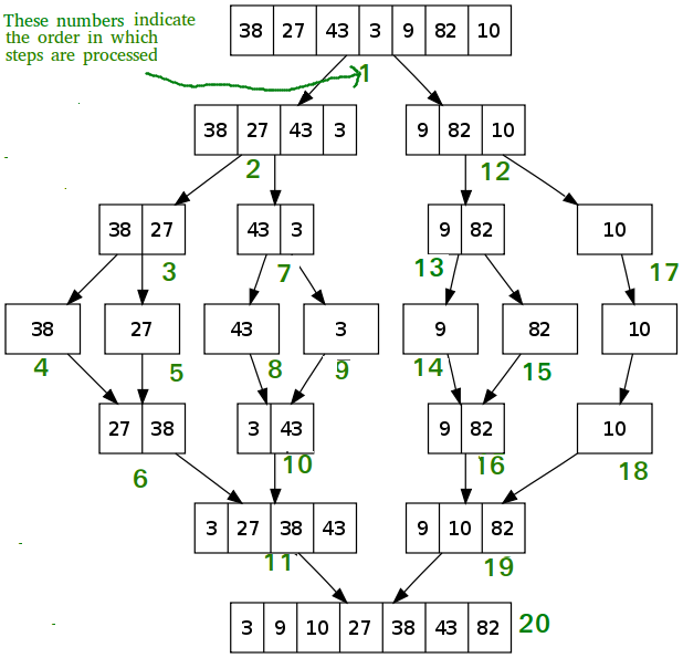
The array breaks down the data until they are all single pieces of data. It then recombines them, moving the lesser to the left and the greater to the right. The sorting is done in this recombine step.
This breaking apart and recombining ensures that the amount of time taken for an operation is as small as possible. The timing will come down to how many times we compare the data. By default, we will compare the data at least n times. We need to look at each number at least once to see where it goes.
The question then arises, how many n times will we have to compare these? It turns out we have to compare it log n number of times. That means we have a runtime of O(nlog n) for the sort.
This log n comes from the fact that we divide the data in half into a tree and therefore only need to do work on the height of that tree. But don’t worry about that right now, we will cover trees in the next lesson.
Like I said, this can be a bit confusing at first. But the main point to understand about this is that mergesort is generally considered a fast sort, and it uses the divide-and-conquer methodology to accomplish its tasks.
Best time: O(nlogn) – The same algorithm is applied no matter what type of array comes in. This means it will always be nlogn.
Average time: O(nlogn) – This is the same as best time.
Worst time: O(nlogn) – This is the same as best time.
Quicksort
Our next algorithm is Quicksort. Quicksort works basically in the same way as mergesort, with one key difference. It uses a “pivot” point to break the data apart. All numbers less than the pivot go to the left, while all numbers greater than the pivot will go to the right.
Quicksort uses the same divide-and-conquer methodology that mergesort does.
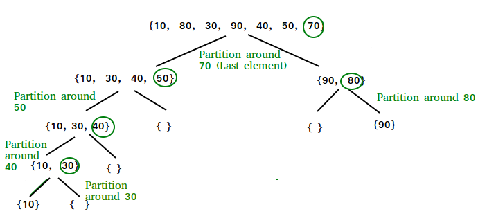
In this particular case, we choose the pivot to be the last number of each group. We then split on that number. So for the first part, 70 is our pivot point. Only 90 and 80 are greater, so they go to the right.
Choosing the pivot point is very important here. If we choose the greatest or least each time, then we don’t really divide the work, and we run into really long run times.
Many times, pivots are chosen by taking three random numbers, and then choosing the one in the middle. This will guarantee that it isn’t the greatest or least when choosing.
Best time: O(nlogn) – This is if we pick a perfect pivot point to split the data. It doesn’t matter if the array comes in sorted or not. The pivot point is what matters the most. If we pick a pivot point that perfectly splits the data each time, then we will have logn levels and therefore, the nlogn run time.
Average time: O(nlogn) – This is if we pick a decent pivot point. As long as we can split up the data and let the program divide and conquer, we get an nlogn time. It won’t be as good as the best, but it will still be nlogn magnitude.
Worst time: O(n^2) – This is if we pick a bad pivot point. Instead of dividing the work up to log(n), we keep only splitting out 1 number each time. The number is larger or smaller than the rest of the array, so we have roughly n levels. Therefore, we end up having the n*n relationship instead of the n*logn relationship.
Key takeaways:
• Mergesort and quicksort are generally determined to be “fast” sorting algorithms.
• They both use divide-and-conquer methodology to split up the work into more efficient chunks.
• Mergesort runs the same no matter what. Quicksort depends on a good pivot point to work effectively.
Tomorrow, we will build off the topics introduced in here and talk about trees.
Cheers,
Kurt
Recommended resources
Mergesort: How mergesort might be implemented with code.
Quicksort: How quicksort might be implemented with code.
Sorting: A great visual resource to see how these sorting algorithms work.
Share with friends