Sorting Algorithms: Part 1
Episode #7 of the course Kurt Anderson by Computer science fundamentals
Welcome back!
Data only means something if we can collect it in a way that can be analyzed. To do this, we typically need sorting. Sorting can be as simple as alphabetical and as complicated as machine-learned AI. Either way, once we have the way we want to sort the problem, we need an algorithm to do the sorting for us.
In today’s lesson, we are going to look at algorithms that are easy to understand but pretty inefficient. Tomorrow, we will look at the more efficient of the bunch.
Bubble Sort
The first algorithm we will look at is bubble sort. This is notoriously the worst sorting algorithm one can use. It starts at the beginning of the data structure, bubbling up the largest number to the end through every pass.
Original: 15, 13, 12, 1, 5
Pass 1: 13, 12, 1, 5, 15
Pass 2: 12, 1, 5, 13, 15
Pass 3: 1, 5, 12, 13, 15
The problem with this algorithm is the run time. It requires us to run through the entire array (n), n amount of times. This means we have an algorithm that is n*n=n^2, which gets really slow.
Best case time: O(n) – This happens if the array is already sorted. It only has to run through the array one time. However, this is a sorting algorithm, so the chance the data is coming in sorted is very low.
Average time: O(n^2) – This run time is calculated because it most likely have to run through the array n/2 times. (Statistically, it will sometimes run less, sometimes run more, but the average is half.) Since the array is length n, this means that it will be n/2*n or n^2 shortened. (Technically, it is (n^2)/2, but we just simplify it.)
Worst time: O(n^2) – This is the same magnitude as average time. Note that average is slightly faster, but we are only concerned with really large differences between algorithms. In its worst case, it will have to run through the n array n number of times (reverse sorted). Since the array is length n, this means that it will be n*n or n^2.
Selection Sort
Selection sort is a little bit more complicated, but arguably just as bad.
The algorithm works by creating two subarrays within a sorting algorithm. The first subarray is the portion that is already sorted. The second is everything that is unsorted.
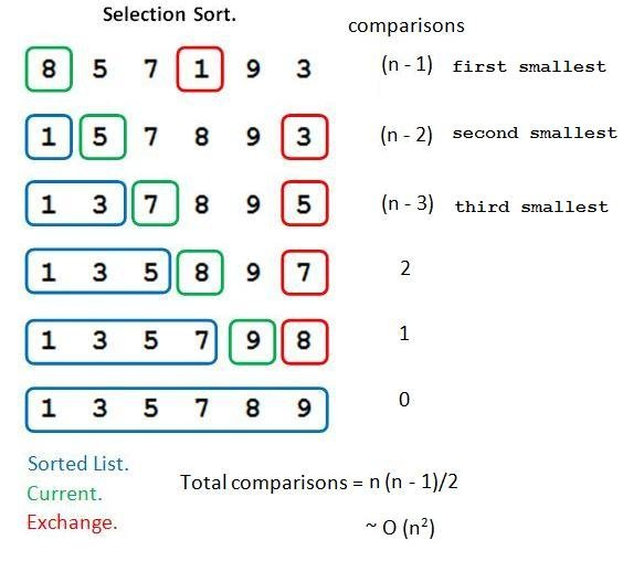
Basically, the algorithm “selects” the smallest number and then inserts it into the “sorted” section of the array. The small improvement this algorithm makes is that it doesn’t start at the beginning of the array each time, giving it a slight boost of speed on bubble sort.
Best time: O(n^2) – This is the cost, though. Even if it’s sorted, it will run at the same amount of time because it still has to “select” each piece of data and put it into the sorted portion.
Average time: O(n^2) – Same as best time, it always has to run through each operation. Even though it’s n^2, it’s a faster n^2 than bubble sort. (We reduce the amount we search after each insertion.)
Worst case time: O(n^2) – Same as average and best times, it always has to run through each operation.
Insertion Sort
Insertion sort works very similar to selection sort. But instead of selecting the smallest number each time, insertion sort takes the number at the beginning of the unsorted portion and “inserts” it into the sorted portion.
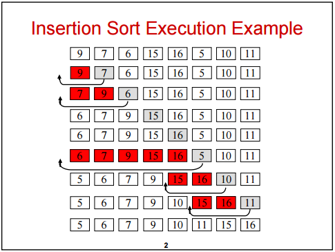
This means it combines the good from selection, with the small speed boost, and the good from bubble, where if already sorted, it can be extremely quick.
Best time: O(n) – If the array comes in sorted, it can do just one pass to figure this out. This makes its best case scenario, an already sorted array, run at n time.
Average time: O(n^2) – On average, we have to search the array one less time each iteration. So, the run time is generally around n(n-1)/2. This means that it will simplify to (n^2-n)/2, which simplifies further to n^2.
Worst time: O(n^2) – This is when the array is reverse sorted. The array will have to insert and swap backward for every single number in the array, making it have to make n operations for the n-sized array. In other words, n*n, which is n^2.
Key takeaway:
• Bubble, selection, and insertion sort are algorithms that might be easy to implement, but they have pretty bad run times.
Tomorrow, we will look at more complicated, but much faster sorting algorithms!
Cheers,
Kurt
Recommended resources
Sorting: A great visual resource to see how these sorting algorithms work.
Share with friends