Simple Linear Regression

Episode #10 of the course Introduction to statistics by Polina Durneva

 

Good morning!

Yesterday, we discussed how to evaluate and analyze the relationship between two categorical variables using the chi-square test. Today, we will talk about how to assess the relationship between two quantitative variables using simple linear regression.

 

Application of Simple Linear Regression

If we have two quantitative variables and we believe that changes in one variable can determine changes in another variable, we can construct a simple linear regression. The simple linear regression takes a form of y = b + k * x, in which we are trying to predict y in terms of x. In the regression, the coefficient k defines the relationship between y and x, and the y-intercept b is the value of y when x is 0.

For instance, you might want to know the relationship between a person’s college GPA and their annual income a year after graduation. In this case, you will use the person’s GPA as an explanatory, or independent, variable and their annual income as an outcome, or dependent, variable. The simple linear regression will take the following form: Annual Income = b + k * (College GPA).

Assuming some fictional dataset, let’s interpret the values of b and k such that Annual Income = 10,000 + 30,000 * (College GPA). The regression means that when a person’s college GPA is 0, their income after graduation is $10,000. (Please note the values are not real and are used only to illustrate the concepts.) Moreover, an increase of college GPA by 1 leads to an increase of annual income by k, or $30,000 in our case.

 

Calculations for Simple Linear Regression

While the interpretation of the coefficients in simple linear regression seems fairly easy, we need to understand how the coefficients and y-intercept are calculated. Consider the following chart that illustrates the data points of our fictional dataset mentioned in the previous section:

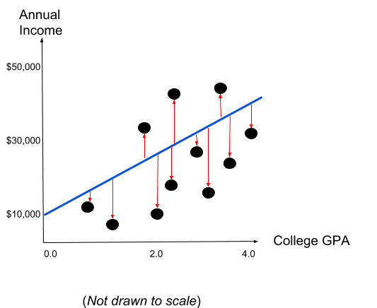
The linear regression is built on the principle of the Least Ordinary Squares. Basically, we are trying to fit a line in the graph with the purpose to minimize the squared distance between the line and each individual observation. Consider the following chart with the best fitted line:

The best fitted line minimizes the sum of the squared residuals (red arrows). Fortunately, nowadays we have different statistical software that can find the best fitted line in less than a second. The residual is squared in order to avoid negative terms that might cancel out positive residuals.

The regression analysis can get more complicated if more independent variables are considered. In this lesson, we talked about the relationship between two quantitative variables. However, it is possible to evaluate the relationship between one variable and a series of other variables. This is called a multiple linear regression. For instance, we can look at the impact of college GPA, family’s income, credit score, and other possible factors on the annual income of a recent graduate. This type of analysis is also based on the Least Ordinary Squares but is more computationally expensive.

That wraps up the course. During the last ten days, we covered the most popular topics that are normally taught during introductory statistics classes. However, I would encourage you to learn more about such an exciting field, expand your knowledge of statistical analysis to other areas, and apply this knowledge to real-world problems.

Thank you and best of luck,

Polina

 

Recommended book

The Black Swan: The Impact of the Highly Improbable by Nassim Nicholas Taleb

 

Share with friends