
Quantitative Variables
Episode #2 of the course Introduction to statistics by Polina Durneva
Hello!
In this lesson, we will discuss quantitative variables. As you may remember from Lesson 1, there are two most popular types of variables: quantitative and categorical. While categorical variables are undoubtedly important, we will focus on the quantitative variables more because of their extensive use in statistics.
Shape and Distribution
If we were to describe any quantitative variable, we would visualize the shape of distribution and analyze it. To visualize any distribution, we can create a dot plot or a histogram.
Assume we have three different datasets that contain information about students’ GPA in three different high schools. Let’s pretend we were able to use a histogram to visualize our data, so we have the following charts (please note that the height of each bar in a histogram is associated with the number of cases, or frequency):
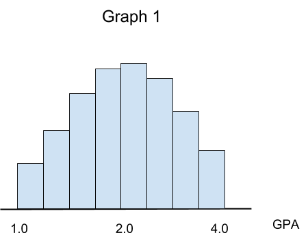
Graph 1 illustrates the distribution of data points for one of our schools. We can see that most students have a GPA of about 2.0, and the distribution looks relatively symmetric. This is an example of a symmetric distribution.
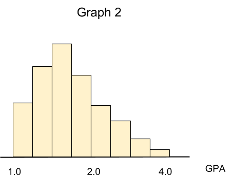
Graph 2 illustrates that most students have a GPA of less than 2.0. This is an example of a skewed to the right distribution.
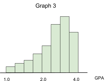
Finally, Graph 3 illustrates a skewed to the left distribution.
Mean and Median
There are two very important measures that can give us an idea of the distribution of data without visualizing it: mean and median.
Mean is a numeric average of all data points in a data set. The formula for mean is: (Sum of all values) / (Number of all values). For population, mean is usually denoted as µ. For a subset of population (sample), mean is usually denoted as x-bar.
Median is the middle value in an ordered array of values. If we have an odd number of values, median is the middle number. For instance, for the set of {1,5,99}, 5 is a median. However, if we have an even number of values, median is an average of the two middle numbers. For instance, for the set {2,5,8,10}, median is (5 + 8) / 2 = 6.5.
If median is equal to mean, the distribution is symmetrical. If median is less than mean, the distribution is skewed to the left; if mean is less than median, the distribution is skewed to the right.
Spread of Data
Another important measure of quantitative variables is the spread of data points. There are three different tools that can be used to evaluate this measure: standard deviation, z-score, and percentile.
Standard deviation demonstrates how far away data points are from the average. High values of standard deviation mean that data points are very spread out.
Moreover, z-score can be quite useful when we want to look at specific data points and the distance of these specific data points from the mean. Standard deviation is used to assess how all points (cases) are spread out, while z-score considers only specific selected data points.
Finally, percentiles are widely used to evaluate both the spread and distribution of data. A certain percentile P of a variable is the value below which a certain percentage of cases fall. For instance, let’s assume that we have 100 students who took a calculus exam: 10% of the students received a score of 100 points (out of 100 points), and the rest received a score less than 100 points. That means 10% of the students are in 90% percentile: These students score better than 90% of all the students in the class.
That’s it for today. Tomorrow, we will talk about confidence intervals.
See you soon,
Polina
Recommended book
Naked Statistics: Stripping the Dread from the Data by Charles Wheelan
Share with friends