P-Values
Episode #5 of the course Introduction to statistics by Polina Durneva
Good morning!
Today, we will discuss p-values, which are very important for evaluation of hypothesis tests.
Hypothesis testing is used primarily to evaluate a claim about population. For instance, if we wanted to know whether the percentage of high school seniors who got into college is higher than 40%, we could set two hypotheses: null hypothesis (the claim that the percentage of high school seniors admitted to college is 40%) and alternative hypothesis (the claim that the percentage of high school students accepted to college is higher than 40%).
The biggest question is: How exactly do we evaluate two hypotheses and find evidence to reject or fail to reject null hypothesis?
That is where p-values come into play!
P-Value
We normally evaluate our hypotheses referring to a random sample from population. Basically, if we find that our sample provides us with an extreme value that is not a coincidence, then we claim to have enough support to reject null hypothesis. However, the biggest challenge here is to prove that our sample value (whether it’s a mean, proportion, or something else we’re testing) is actually an evidence against null hypothesis and not some kind of an outlier that happened to represent our sample.
The p-value is very important here. The p-value is the probability of getting an observed value (or an extreme value) from our sample, given that null hypothesis is true. Let’s refer to our example of high school seniors to understand the concept better.
Our null hypothesis is that the percentage of high school seniors accepted to college is 40%, and our alternative hypothesis is that the percentage of high school seniors admitted to college is higher than 40%. Our alternative hypothesis is based on our random sample in which we found that the percentage of high school students accepted to college is higher than 40% (i.e., 50%). Let’s assume we find the p-value of 0.05. This p-value means that the probability that our sample result (p > 0.4) could happen by random chance is 5%. On the other hand, if we had the p-value of 0.9, it would mean that the probability of our result to be random is 90%.
As you can see from the previous example, lower p-values are better if we seek to reject null hypothesis and find enough evidence to support alternative hypothesis. Statisticians usually consider the p-value of 0.05 or lower to be a strong evidence to reject null hypothesis. However, the cutoff for the p-values is subjectively based on the nature of a study and other factors.
Calculation of P-Value
To calculate the p-value, statisticians use a randomization distribution assuming that null hypothesis is true. Creating a randomization distribution requires finding more samples from the population of our interest or using a computer simulation.
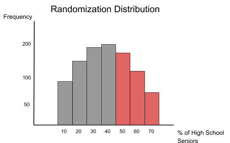
In the above example, we talked about high school seniors admitted to college. Our alternative hypothesis was based on a fictional sample in which the percentage of high school seniors accepted to college was larger than 40%. To create a randomization distribution, we need to get more samples of high school seniors and check the number of students admitted to college in each sample. Ideally, we would want to have thousands of samples for a better accuracy. Let’s assume that we were able to get 1,000 different samples of high school seniors and created a randomization distribution that displays the percentage of students admitted to college:

In total, we have 1,000 samples. We are interested in the red bars on the right because these are the samples that have the percentages of high school seniors accepted to college higher than 40%. Let’s assume that the frequencies for these three bars are 190, 150, and 80 (meaning that 190 samples have 50% of the high school students admitted to college, 150 samples have 60%, and 80 samples have 70%). Don’t forget that the total number of samples is 1,000.
The p-value is the sum of the samples that have extreme values (>40%) divided by the total number of samples. Thus, our p-value is: (190 + 150 + 80) / 1000 = 0.42. It means that the probability of our extreme values (>40%) to be random (assuming that null hypothesis is true) is 42%. This value is large enough to fail to reject null hypothesis, since all our samples with values higher than 40% could have happened by chance and have no statistical significance.
That’s it for today. Tomorrow, we will talk about Central Limit Theorem and normal distribution.
Thank you,
Polina
Recommended book
What is a p-value anyway? 34 Stories to Help You Actually Understand Statistics by Andrew J. Vickers
Share with friends

