Linked Lists
Episode #5 of the course Kurt Anderson by Computer science fundamentals
Welcome back!
Yesterday, we saw our first data structure, the array. However, it had the shortcoming of being locked to a certain size. Today, we are going to look at a data structure that can expand indefinitely: the linked list.
What Are Linked Lists?
Linked lists work through the use of pointers. Pointers are just elements that store the location of another element.
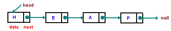
In the example above, we can see this in action. The first element in a linked list is called the head. Whenever we call the linked list, it will point to this head element.
In computer science, we call these entities, nodes. A node is a special element like a package. It holds the main data and then “metadata,” which are just other helpful pieces of data.
In a linked list, each node holds the original data and then a pointer to the next node. Each further node does the exact same thing until the end of the list is reached. This ending is signified by the special null character, which just means “nothing” in computer science.
How Are They Different from Arrays?
The major difference with this data structure is that it can expand indefinitely. No size has to be declared upon creation.
Remember how arrays could run into the problem where they had unused space? For example, if an array has 200 elements, but only 25 are filled, 175 go to waste. Linked lists don’t run into this problem. They only use the space they need. With a linked list, you just need to add to the end with each new piece of data. So, a linked list with 25 elements will use 25 pieces of data. There is never any data waste with them.
Now, this comes at some costs. With arrays, we could access all the elements in constant time. So, the first element, the middle element, and the last element could all be accessed at the same time. With a linked list, however, since each element is linked to the previous one, we have to travel through the list each time we want to access an element. For example, if we want to access the fourth element, we have to travel through four nodes to get to that element. This can increase the run times we discussed with array.
Linked List Run Times
Insert (random): O(n) – To insert at a particular location, one has to traverse the list up to that point to insert there. Since this could be near the end, we say the worst case is the entire list, or n.
Insert (front): O(1) – We just move the head pointer to the new node and point the new node at the old head.
Insert (back): O(n) – We will have to traverse the entire array to get to the back. (We can create a pointer that always points to the back to reduce this to constant time. It’s called a “tail pointer.”)
Delete (random): O(n) – We must traverse the length of the element we want to delete. Since this could be near the end, we say the worst case is the entire list, or n.
Delete (front): O(1) – As easy as inserting, we just have to remove the first element and repoint the head pointer to the next element.
Search (sorted): O(n) – It doesn’t matter if it’s sorted or not. At worst, we have to traverse the entirety of the list to find the element. (And if the element isn’t in the list, we have to traverse the entire list to figure that out.)
Search (unsorted): O(n) – This is exactly the same as the Sorted.
Key takeaways:
• Linked lists are data structures that can expand indefinitely.
• Linked lists use nodes linked together with pointers.
• This comes at a time cost, i.e., increases the time it takes to find elements that aren’t the first element.
• Linked lists use only the space they need.
Tomorrow, we will build new data structures with linked lists!
Cheers,
Kurt
Recommended resources
Linked Lists: More visual representations of how linked lists work.
Linked List Data Structure: Example code of how a linked list might be implemented.
Share with friends