
Confidence Intervals
Episode #3 of the course Introduction to statistics by Polina Durneva
Good morning!
Today, you’ll learn about confidence intervals. But before that, we need to have a clear understanding of the difference between parameters and statistics.
Parameters vs. Statistics
Parameters are used to describe population, while statistics are used to describe samples from population. In Lesson 1, we used an example of a fast food restaurant in which we wanted to find the proportion of customers who buy burgers and fries and the proportion of customers who buy chicken wings. If we were to ask each single customer about their choice of food, we would have an exact value that demonstrates how many customers buy one type of meal or another. This value would be our parameter, as it describes the entire population of our fast food restaurant.
However, it would be quite a tedious and tiring process to survey each customer, and therefore, we agreed to choose a sample of random customers and ask them about their choice of meals. We would have a random sample that would provide us with a statistic, which approximates the parameter. Statistics are used to provide us with the estimation of parameters.
Margin of Error
To have a better estimation of a parameter with respect to a statistic, statisticians come up with a margin of error. Using a margin of error, we can have an interval that provides us with a range of values, one of which is a parameter. A margin of error is calculated using multiple samples: More different samples provide us with a lower value of an error and a more accurate estimation of a statistic.
For instance, let’s assume that our estimated statistic for customers who prefer chicken wings is 30%, meaning that 30% of the clients in our fast food restaurant prefer chicken wings to burgers with fries. An estimated margin of error is 5%, meaning that our parameter would be any value between 25% and 35%.
Confidence Interval
We can also add some features to the aforementioned interval, which is based on a statistic and a margin of error, and redefine it as a confidence interval, which is a range of plausible values. However, sometimes we might get a statistic that is biased and does not capture a parameter even with a margin of error. To evaluate that, statisticians came up with something called the confidence level. The confidence level is the probability of the confidence interval to capture a population parameter.
Most of the time, statisticians use a 95% confidence interval. To better understand it, look at the graph below:
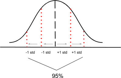
The graph illustrates a bell-shaped distribution: 95% of the distribution roughly lies within two standard deviations of the center of the distribution. Therefore, it is assumed that a population parameter lies within two standard deviations—or standard errors, in this case—within the center. The formula for a 95% confidence interval would be: (Statistic – 2 * (Standard Error)); (Statistic + 2 * (Standard Error)).
For example, let’s say that we want to estimate the percentage of high school seniors who got accepted to college in state X. After getting a random sample of high school students, we get 76%. We also know that the standard error is 4.5%. Thus, our confidence interval would be, (76% – 2 * 4.5%; 76% + 2 * 4.5%) = (67%; 85%), meaning that we can be 95% sure that between 67% and 85% of high school seniors in state X got accepted to college.
That’s it for today. Tomorrow, we will discuss hypothesis tests.
See you,
Polina
Recommended book
Share with friends