
Central Limit Theorem and Normal Distribution
Episode #6 of the course Introduction to statistics by Polina Durneva
Hello!
Today, we will talk about a couple of important statistical concepts: normal distribution and Central Limit Theorem.
Normal Distribution
For any statistical analysis, it is good to use as many samples of population as possible. For instance, if you want to know the percentage of people who prefer winter to summer, you need to ask random groups of people about their preference. Once you get opinions of 30 people or more (it is preferred to have a sample size of at least 30 observations), you can call this group of people a sample.
Then, you can create another sample consisting of other 30 random people and so on. For each sample, you will have a certain statistic: a proportion of people who like winter more than summer, for example. If the number of your samples is large enough, all statistics you collected will create a bell-shaped, symmetrical distribution. This is a normal distribution.
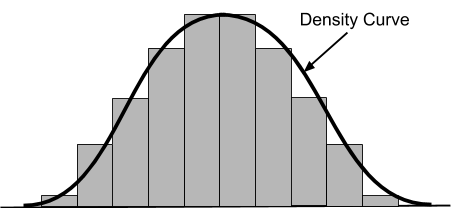
Density Curve
Normal distributions are closely associated with a density curve, which is a line following the shape of a distribution. The chart below illustrates a normal distribution and a density curve:
The most important characteristics of the normal density curve are mean, median, and standard deviation. The normal density curve is denoted as N(μ,σ), where μ is the mean and σ is the standard deviation. For statistical purposes, the normal density curve is converted on the scale from -1 and 1, such that the mean becomes 0 and the standard deviation becomes 1.
It is important to note that the area under the curve adds up to 1. If we look at certain intervals of the distribution, the area under the curve represents the probability of such intervals in the population.
For instance, let’s say we want to know the percentage of people who prefer winter to summer. What is the probability that the percentage of people who prefer winter to summer is between 70% and 80%? Consider the following chart:
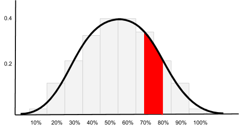
As you can see, the area below the density curve over the interval of our interest is in red. Approximately, we would get the area of 0.06, and this is the probability of what we are looking for.
Central Limit Theorem
Normal distribution tends to center at its mean value (or a population parameter). It was statistically proven that for a large number of samples, the center of a normal distribution does center at the value of the parameter we are looking for. This is the main idea behind Central Limit Theorem.
For instance, if we were to look at the percentage of people who prefer winter to summer, the real percentage that represents the entire population would be at the center of our normal distribution.
Consider the following chart based on the above example:
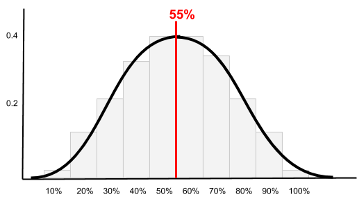
Assume we have 1,000 different samples, and the percentage of those who like winter is 55% (the peak of the curve) for the majority of our samples. Thus, this value (or approximately this value) is representative of the entire population.
That’s it for today! Tomorrow, we will discuss degrees of freedom.
Take care,
Polina
Recommended book
Statistics Done Wrong: The Woefully Complete Guide by Alex Reinhart
Share with friends